Keras入门（二）模型的保存、读取及加载

本文将会介绍如何利用Keras来实现模型的保存、读取以及加载。

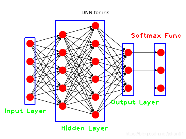
本文使用的模型为解决IRIS数据集的多分类问题而设计的深度神经网络（DNN）模型，模型的结构示意图如下：

模型保存

Keras使用HDF5文件系统来保存模型。模型保存的方法很容易，只需要使用save()方法即可。

以Keras入门（一）搭建深度神经网络（DNN）解决多分类问题中的DNN模型为例，整个模型的变量为model，我们设置模型共训练10次，在原先的代码中加入Python代码即可保存模型：

# save model
print("Saving model to disk \n")
mp = "E://logs/iris_model.h5"
model.save(mp)

保存的模型文件（iris_model.h5）如下：

模型读取

保存后的iris_model.h5以HDF5文件系统的形式储存，在我们使用Python读取h5文件里面的数据之前，我们先用HDF5的可视化工具HDFView来查看里面的数据：

我们感兴趣的是这个模型中的各个神经层之间的连接权重及偏重，也就是上图中的红色部分，model_weights里面包含了各个神经层之间的连接权重及偏重，分别位于dense_1,dense_2,dense_3中。蓝色部分为dense_3/dense_3/kernel:0的数据，即最后输出层的连接权重矩阵。

有了对模型参数的直观认识，我们要做的下一步工作就是读取各个神经层之间的连接权重及偏重。我们使用Python的h5py这个模块来这个iris_model.h5这个文件。关于h5py的快速入门指南，可以参考文章：h5py快速入门指南。

使用以下Python代码可以读取各个神经层之间的连接权重及偏重数据：

import h5py

# 模型地址
MODEL_PATH = 'E://logs/iris_model.h5'

# 获取每一层的连接权重及偏重
print("读取模型中...")
with h5py.File(MODEL_PATH, 'r') as f:
    dense_1 = f['/model_weights/dense_1/dense_1']
    dense_1_bias =  dense_1['bias:0'][:]
    dense_1_kernel = dense_1['kernel:0'][:]

    dense_2 = f['/model_weights/dense_2/dense_2']
    dense_2_bias = dense_2['bias:0'][:]
    dense_2_kernel = dense_2['kernel:0'][:]

    dense_3 = f['/model_weights/dense_3/dense_3']
    dense_3_bias = dense_3['bias:0'][:]
    dense_3_kernel = dense_3['kernel:0'][:]

print("第一层的连接权重矩阵：\n%s\n"%dense_1_kernel)
print("第一层的连接偏重矩阵：\n%s\n"%dense_1_bias)
print("第二层的连接权重矩阵：\n%s\n"%dense_2_kernel)
print("第二层的连接偏重矩阵：\n%s\n"%dense_2_bias)
print("第三层的连接权重矩阵：\n%s\n"%dense_3_kernel)
print("第三层的连接偏重矩阵：\n%s\n"%dense_3_bias)

输出的结果如下：

读取模型中...
第一层的连接权重矩阵：
[[ 0.04141677  0.03080632 -0.02768146  0.14334357  0.06242227]
 [-0.41209617 -0.77948487  0.5648218  -0.699587   -0.19246106]
 [ 0.6856315   0.28241938 -0.91930366 -0.07989818  0.47165248]
 [ 0.8655262   0.72175753  0.36529952 -0.53172135  0.26573092]]

第一层的连接偏重矩阵：
[-0.16441862 -0.02462054 -0.14060321  0.         -0.14293939]

第二层的连接权重矩阵：
[[ 0.39296603  0.01864707  0.12538083  0.07935872  0.27940807 -0.4565802 ]
 [-0.34312084  0.6446907  -0.92546445 -0.00538039  0.95466876 -0.32819661]
 [-0.7593299  -0.07227057  0.20751365  0.40547106  0.35726753  0.8884158 ]
 [-0.48096     0.11294878 -0.29462305 -0.410536   -0.23620337 -0.72703975]
 [ 0.7666149  -0.41720924  0.29576775 -0.6328017   0.43118536  0.6589351 ]]

第二层的连接偏重矩阵：
[-0.1899569   0.         -0.09710662 -0.12964155 -0.26443157  0.6050924 ]

第三层的连接权重矩阵：
[[-0.44450542  0.09977101  0.12196152]
 [ 0.14334357  0.18546402 -0.23861367]
 [-0.7284191   0.7859063  -0.878823  ]
 [ 0.0876545   0.51531947  0.09671918]
 [-0.7964963  -0.16435687  0.49531657]
 [ 0.8645698   0.4439873   0.24599855]]

第三层的连接偏重矩阵：
[ 0.39192322 -0.1266532  -0.29631865]

值得注意的是，我们得到的这些矩阵的数据类型都是numpy.ndarray。

OK，既然我们已经得到了各个神经层之间的连接权重及偏重的数据，那我们能做什么呢？当然是去做一些有趣的事啦，那就是用我们自己的方法来实现新数据的预测向量(softmax函数作用后的向量)。so, really?

新的输入向量为[6.1, 3.1, 5.1, 1.1]，使用以下Python代码即可输出新数据的预测向量：

import h5py
import numpy as np

# 模型地址
MODEL_PATH = 'E://logs/iris_model.h5'

# 获取每一层的连接权重及偏重
print("读取模型中...")
with h5py.File(MODEL_PATH, 'r') as f:
    dense_1 = f['/model_weights/dense_1/dense_1']
    dense_1_bias =  dense_1['bias:0'][:]
    dense_1_kernel = dense_1['kernel:0'][:]

    dense_2 = f['/model_weights/dense_2/dense_2']
    dense_2_bias = dense_2['bias:0'][:]
    dense_2_kernel = dense_2['kernel:0'][:]

    dense_3 = f['/model_weights/dense_3/dense_3']
    dense_3_bias = dense_3['bias:0'][:]
    dense_3_kernel = dense_3['kernel:0'][:]

# 模拟每个神经层的计算，得到该层的输出
def layer_output(input, kernel, bias):
    return np.dot(input, kernel) + bias

# 实现ReLU函数
relu = np.vectorize(lambda x: x if x >=0 else 0)

# 实现softmax函数
def softmax_func(arr):
    exp_arr = np.exp(arr)
    arr_sum = np.sum(exp_arr)
    softmax_arr = exp_arr/arr_sum
    return softmax_arr

# 输入向量
unkown = np.array([[6.1, 3.1, 5.1, 1.1]], dtype=np.float32)

# 第一层的输出
print("模型计算中...")
output_1 = layer_output(unkown, dense_1_kernel, dense_1_bias)
output_1 = relu(output_1)

# 第二层的输出
output_2 = layer_output(output_1, dense_2_kernel, dense_2_bias)
output_2 = relu(output_2)

# 第三层的输出
output_3 = layer_output(output_2, dense_3_kernel, dense_3_bias)
output_3 = softmax_func(output_3)

# 最终的输出的softmax值
np.set_printoptions(precision=4)
print("最终的预测值向量为: %s"%output_3)

其输出的结果如下：

1
2
3

读取模型中...
模型计算中...
最终的预测值向量为: [[0.0242 0.6763 0.2995]]

额，这个输出的预测值向量会是我们的DNN模型的预测值向量吗？这时候，我们就需要回过头来看看Keras入门（一）搭建深度神经网络（DNN）解决多分类问题中的代码了，注意，为了保证数值的可比较性，笔者已经将DNN模型的训练次数改为10次了。让我们来看看原来代码的输出结果吧：

Using model to predict species for features: 
[[6.1 3.1 5.1 1.1]]

Predicted softmax vector is: 
[[0.0242 0.6763 0.2995]]

Predicted species is: 
Iris-versicolor

Yes,两者的预测值向量完全一致！因此，我们用自己的方法也实现了这个DNN模型的预测功能，棒！

模型加载

当然，在实际的使用中，我们不需要再用自己的方法来实现模型的预测功能，只需使用Keras给我们提供好的模型导入功能（keras.models.load_model()）即可。使用以下Python代码即可加载模型

# 模型的加载及使用
from keras.models import load_model
print("Using loaded model to predict...")
load_model = load_model("E://logs/iris_model.h5")
np.set_printoptions(precision=4)
unknown = np.array([[6.1, 3.1, 5.1, 1.1]], dtype=np.float32)
predicted = load_model.predict(unknown)
print("Using model to predict species for features: ")
print(unknown)
print("\nPredicted softmax vector is: ")
print(predicted)
species_dict = {v: k for k, v in Class_dict.items()}
print("\nPredicted species is: ")
print(species_dict[np.argmax(predicted)])

输出结果如下：

Using loaded model to predict...
Using model to predict species for features: 
[[6.1 3.1 5.1 1.1]]

Predicted softmax vector is: 
[[0.0242 0.6763 0.2995]]

Predicted species is: 
Iris-versicolor