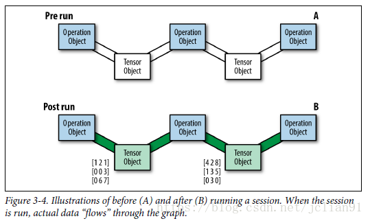
TensorFlow optimizes its computations based on the graph’s
connectivity.
Each graph has its own set of node dependencies.Being able to locate
dependencies between units of our model allows us to both distribute
computations across available resources and avoid performing redundant
computations of irrelevant subsets, resulting in a faster and more
efficient way of computing things.
Variables
Variables are constructs in TensorFlow that allows us to store and
update parameters of our models in the current session during training.
To define a “variable” tensor, we use TensorFlow’s Variable()
constructor. to execute a computational graph that contains variables,
we must initialize all variables in the active session first (using
tf.global_variables_initializer()).
例1:使用Variables
1 2 3 4 5 6 7 8 9 10 11 12 13 14 15 16 17
import tensorflow as tf
g = tf.Graph() with g.as_default() as g: tf_x = tf.Variable([[1., 2.], [3., 4.], [5., 6.]], dtype=tf.float32) x = tf.constant(1., dtype=tf.float32)
# add a constant to the matrix: tf_x = tf_x + x
with tf.Session(graph=g) as sess: sess.run(tf.global_variables_initializer()) result = sess.run(tf_x)
print(result)
输出结果:
1 2 3
[[2. 3.] [4. 5.] [6. 7.]]
例2: 运行两遍?
运行两遍, 存在的问题:
1 2 3 4 5 6 7 8 9 10 11 12 13 14 15 16 17 18
import tensorflow as tf
g = tf.Graph() with g.as_default() as g: tf_x = tf.Variable([[1., 2.], [3., 4.], [5., 6.]], dtype=tf.float32) x = tf.constant(1., dtype=tf.float32)
# add a constant to the matrix: tf_x = tf_x + x
with tf.Session(graph=g) as sess: sess.run(tf.global_variables_initializer()) result = sess.run(tf_x) result = sess.run(tf_x) # 运行两遍
print(result)
输出结果:
1 2 3
[[2. 3.] [4. 5.] [6. 7.]]
解决办法? 使用tf.assign()函数。
1 2 3 4 5 6 7 8 9 10 11 12 13 14 15 16 17 18
import tensorflow as tf
g = tf.Graph() with g.as_default() as g: tf_x = tf.Variable([[1., 2.], [3., 4.], [5., 6.]], dtype=tf.float32) x = tf.constant(1., dtype=tf.float32)
# add a constant to the matrix: update_tf_x = tf.assign(tf_x, tf_x + x)
with tf.Session(graph=g) as sess: sess.run(tf.global_variables_initializer()) result = sess.run(update_tf_x) result = sess.run(update_tf_x) # 运行两遍
print(result)
此时的输出结果:
1 2 3
[[3. 4.] [5. 6.] [7. 8.]]
Placeholder Variables
Placeholder variables allow us to feed the
computational graph with numerical values in an active session at
runtime. Placeholders have an optional shape argument.
If a shape is not fed or is passed as None, then the
placeholder can be fed with data of any size.
例:矩阵相乘
指定行数与列数
1 2 3 4 5 6 7 8 9 10 11 12 13 14 15 16 17
import tensorflow as tf import numpy as np
g = tf.Graph() with g.as_default() as g: tf_x = tf.placeholder(dtype=tf.float32,shape=(3, 2))
# initialize a Saver, which gets all variables # within this computation graph context saver = tf.train.Saver()
with tf.Session(graph=g) as sess: sess.run(tf.global_variables_initializer()) result = sess.run(update_tf_x)
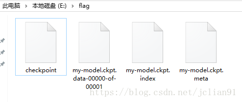
# save the model saver.save(sess, save_path='E://flag/my-model.ckpt')
保存的文件:
保存的文件
The file my-model.ckpt.data-00000-of-00001 saves our main variable
values, the .index file keeps track of the data structures, and the
.meta file describes the structure of our computational graph that we
executed.
# initialize a Saver, which gets all variables # within this computation graph context saver = tf.train.Saver()
with tf.Session(graph=g) as sess: saver.restore(sess, save_path='E://flag/my-model.ckpt') result = sess.run(update_tf_x) print(result)
运行结果:
1 2 3
[[3. 4.] [5. 6.] [7. 8.]]
Naming TensorFlow Objects
Each Tensor object also has an identifying name. This name is an
intrinsic string name, not to be confused with the name of the variable.
As with dtype, we can use the .name attribute to see the name of the
object:
1 2 3 4 5 6 7 8 9
import tensorflow as tf
g = tf.Graph() with g.as_default() as g: c1 = tf.constant(4, dtype=tf.float64, name='c') c2 = tf.constant(4, dtype=tf.int32, name='c')
print(c1.name) print(c2.name)
输出:
1 2
c:0 c_1:0
Name scopes
Sometimes when dealing with a large, complicated graph, we would like
to create some node grouping to make it easier to follow and manage. For
that we can hierarchically group nodes together by name. We do so by
using tf.name_scope("prefix") together with the useful with clause
again:
1
2
3
4
5
6
7
8
9
10
11
12
import tensorflow as tf
g = tf.Graph() with g.as_default() as g: c1 = tf.constant(4, dtype=tf.float64, name='c') with tf.name_scope("prefix_name"): c2 = tf.constant(4, dtype=tf.int32, name='c') c3 = tf.constant(4, dtype=tf.float64, name='c')
print(c1.name) print(c2.name) print(c3.name)
输出:
1 2 3
c:0 prefix_name/c:0 prefix_name/c_1:0
CPU and GPU
All TensorFlow operations in general, can be executed on a
CPU. If you have a GPU version of
TensorFlow installed, TensorFlow will automatically execute those
operations that have GPU support on GPUs and use your
machine’s CPU, otherwise.
Control Flow
例: if-else结构
简单的if-else语句
1 2 3 4 5 6 7 8 9 10 11 12 13 14 15 16
import tensorflow as tf
addition = True
g = tf.Graph() with g.as_default() as g: x = tf.placeholder(dtype=tf.float32, shape=None) if addition: y = x + 1. else: y = x - 1.
with tf.Session(graph=g) as sess: result = sess.run(y, feed_dict={x: 1.})
print('Result:\n', result)
输出:
1 2
Result: 2.0
使用tf.cond()代替上面的if-else语句
1 2 3 4 5 6 7 8 9 10 11 12 13 14 15
import tensorflow as tf
g = tf.Graph() with g.as_default() as g: addition = tf.placeholder(dtype=tf.bool, shape=None) x = tf.placeholder(dtype=tf.float32, shape=None)
y = tf.cond(addition, true_fn=lambda: tf.add(x, 1.), false_fn=lambda: tf.subtract(x, 1.))
with tf.Session(graph=g) as sess: result = sess.run(y, feed_dict={addition:True,x: 1.})
print('Result:\n', result)
输出结果:
1
2
Result:
 2.0
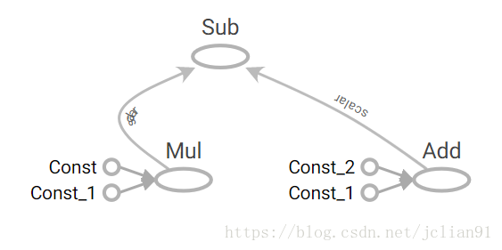
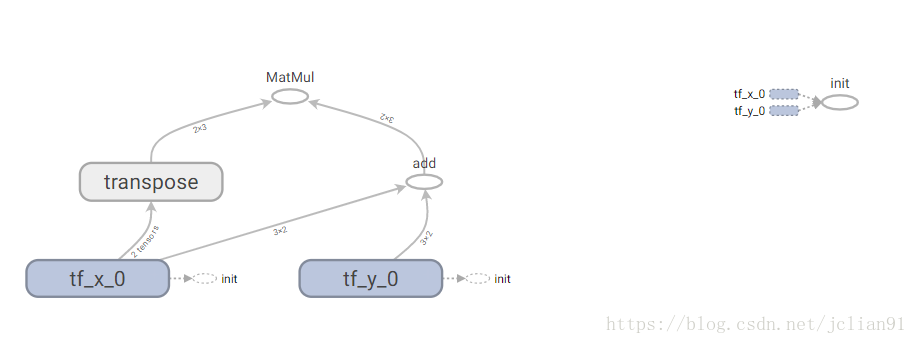
TensorBoard
TensorBoard is one of the coolest features of TensorFlow, which
provides us with a suite of tools to visualize our computational graphs
and operations before and during runtime.
# -*- coding: utf-8 -*- import pandas as pd import numpy as np import tensorflow as tf from sklearn.linear_model import LogisticRegression
#read data from other places, e.g. csv #drop_list: variables that are not used defread_data(file_path, drop_list=[]): dataSet = pd.read_csv(file_path,sep=',') for col in drop_list: dataSet = dataSet.drop(col,axis=1) return dataSet
# tensorflow训练模型 with g.as_default(): x = tf.placeholder(tf.float32, shape=[None, var_num]) y_true = tf.placeholder(tf.float32, shape=None)
with tf.name_scope('inference') as scope: w = tf.Variable([[-1]*var_num], dtype=tf.float32, name='weights') b = tf.Variable(0, dtype=tf.float32, name='bias') y_pred = tf.matmul(w, tf.transpose(x)) + b
with tf.name_scope('train') as scope: # labels: ture output of y, i.e. 0 and 1, logits: the model's linear prediction cross_entropy = tf.nn.sigmoid_cross_entropy_with_logits(labels=y_true, logits=y_pred) loss = tf.reduce_mean(cross_entropy)